Top Excel time-saving tips

Excel has masses of features, so picking out just 5 isn't easy.  But here are a few which you may not have come across.  Give them a try; you'll wonder how you ever managed without them!

1. Sum without a formula

If you want to see a quick total of a range of values without having to put a formula in (e.g. as a quick check), highlight the range then take a look at the bottom of the Excel window.

 

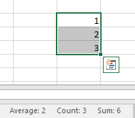
You'll see the Average, Count and Sum of the values you highlighted.  You can right-click on the bottom bar to see more options such as Maximum, Minimum; just tick the ones you would like to see.

2. Quick Navigation

Instead of using scroll bars or arrow keys to move around the spreadsheet, you can use short cut keys to go to the top or bottom

Ctrl+Home takes you to cell A1

Ctrl+End takes you to the bottom right used cell

Ctrl+Down Arrow takes you to the last cell in the column

Ctrl+Right Arrow takes you to the last cell in the row

3. Set Column Width

You can manually set columns to the width of your text, but a really quick way to do this is to select the column (click on the column letter), then move your cursor over to the right until you see a small black cross.  Double click while this is displayed and hey presto, the column will be automatically the same width as the longest text in that column.

You can do the same thing with rows, but this will only work if you don't have wrapped text.

4. Keep headings visible

If you have a large spreadsheet, when you scroll down or across you can no longer see the column headings or row information.  To keep these visible, you can use the Freeze Panes option.

First select the cell on row below your column headings and one column to the right of the rows you want to keep visible.  Then go to the "View" tab on the ribbon and select the "Freeze Panes" option.

 

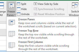
Click on the Freeze Panes option to keep the columns above and rows to the left of the cell you selected visible even if you navigate further down or across the page.

5. Format Painter

This useful tool is often overlooked but is really great if you have formatted some cells as currency for example and want to apply that formatting to other areas.

Select the cell that has the formatting you want and click on the Format Painter on the Home tab of the ribbon

 

Now click on the cell(s) where you want to apply the same formatting.  When you release the mouse button the format will automatically be applied.